Intergenerational Value of Farmland Applied Biochar

The intergenerational value of farmland biochar can be profound, yet it is poorly represented, if at all.  Biochar carbon removal is a well recognized climate service now.  But the tangible values of the physical product are a different story.  We generally consider the value biochar material as determined by its sale price, which may or may not have anything to do with the benefits to humanity that will be generated from that biochar over the course of it’s lifetime.

Ultimately, biochar can increase the carrying capacity of farmlands where it is applied, and over the course of a few centuries, the cumulative value of this is immense.  Problem: what metrics would that be measured in?  To help move the conversation forward, I’ve suggested a few metrics that you’ll find in this article and the worksheet I am now open-sourcing here.

Here are some key takeaways regarding intergenerational value:

1. Market price of the physical biochar material grossly underrepresents the intrinsic value to humanity when farmland applied.

2. The GENERATIONAL value of biochar that is farmland applied, in terms of crop increase alone, is greater than the CDR price we are paying to put it there.

3. The INTERGENERATIONAL value of biochar that is farmland applied, in terms of crop increase alone, is an order of magnitude greater than the CDR price we are paying to put it there.*

   *as determined by average of crops measured, conservatively excluding strawberries, and looking at the values of generational (20 yrs) and intergenerational (1,000 yrs) timelines, respectively, while applying 2% discount rate.

Here are some key takeaways regarding ROI and market development for biochar as a farmland improvement:

1. Farmland owners stand to benefit from the increased availability of biochar.

2. Crops with high value per acre, and where soil health deficiencies are present, stand to financially benefit the greatest.

3. In some cases, water conservation alone can provide a positive ROI on a biochar investment.

The model is not globally comprehensive, not yet at least.  I built it for our own market development purposes within Pacific Biochar, and we’re primarily producing biochar in California, so that’s about the regional extent of what we’ve looked at.  I’ve shared it in an editable form so you can use it for your own purposes, and I hope you do.

Biochar is two products really, a carbon removal service and a physical material that is mostly used in farmland improvement.  These two products have an interesting interplay.  Put simply, the carbon removal service cannot be complete until the physical material has been safely sequestered in the soil.

The carbon removal service can be sold internationally, and the bulky physical material usually stays within the region of production.

In order to optimize the regional distribution of the physical biochar material, I’ve leaned on a specific tool to help me identify markets.  It has evolved into the spreadsheet I’m sharing here.   The underlying assumption is that if the land owner, by purchasing and applying biochar, can get a significantly positive return on investment (ROI) in less than 5 harvests, it’s a potentially viable market.  The next step, and this one can take years of field trials to achieve, is that the land owners must have sufficient confidence that the biochar applications will in fact deliver results as desired.

ROI analysis for biochar applications to California almond crop, per average yield data of year 2023

So, in a nutshell, that’s the core function of the ROI analysis.  As you’ll see in the spreadsheet, a few things come clear, all else equal, the crop’s revenue per acre is one of the most critical determining factors; the higher the revenue per acre, the faster the path to a positive ROI.

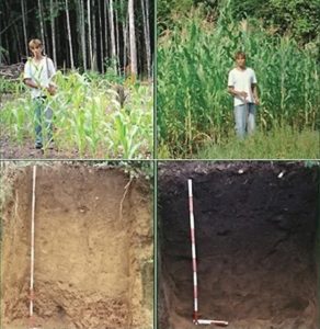
Terra Preta soil on right, parent soil on left

But… after a while, I began looking at these numbers in a different way.  The biochar we apply today will continue providing biochar far beyond our lifetimes, such as in the case of the iconic Terra Preta soils of the Amazon region.

 Biochar that improves farmland soils can be considered an asset that continues to generate a marginal increase in revenue as long as the soils are actively farmed.  So, I adapted the financial concept of net present value (NPV) to farmland applications of biochar to help me better understand the intergenerational values of what we’re doing.

Definition of Net Present Value from Wikipedia:
The net present value (NPV) or net present worth (NPW) is a way of measuring the value of an asset that has cashflow by adding up the present value of all the future cash flows that asset will generate. The present value of a cash flow depends on the interval of time between now and the cash flow because of the Time value of money (which includes the annual effective discount rate). It provides a method for evaluating and comparing capital projects or financial products with cash flows spread over time, as in loans, investments, payouts from insurance contracts plus many other applications.

Intergenerational value is perhaps a more apt term instead of NPV in this scenario, because NPV is explicitly designed to look at things from the perspective of the present.  Essentially NPV is asking “over the lifetime of this asset, what is its value to ME”.  However, the incredibly long timelines we’re dealing with in this case are a stretch beyond the generations alive today, and therefore a perhaps a stretch beyond what the NPV is commonly intended for.  We can toggle back and forth on this topic though, because it’s a really important consideration in determining what discount rate should be applied, and the discount rate has a huge impact on the values calculated.

Projected intergenerational value of biochar applications in California almond crop, per average yield data of year 2023

The model is preset with input values that you can change yourself if you desire.  Here’s some notes on the preset values:

I added conditional formatting on each page, which makes all numerical inputs show as blue, and all calculated values show as black.  If you see a number with blue font, it’s an input.

Crop metrics are preset with the most recent year’s data.  I did not take long-term averages, I took only the data from the most recent year’s average acreage, yield, and price.  Crop yield per acre and price per pound can vary a lot year to year, so this is important to note.  For instance, the crop metrics for CA Walnuts show some dismal numbers, as the year I took data from was an historically tough year for that crop.

Yield increase due to biochar application is assumed at 10%.

The assumed crop yield increase of 10% is based on a global meta-analysis (Ye et al, 2020, referenced in worksheet) in which a very wide variety of soil types and crop types are represented. This 10% crop yield increase is the more conservative of numbers that one could choose from in looking at global average crop yield increase, and is the number that I believe best represents the majority of applications because it is specifically excluding comparisons of biochar vs control where no other fertilizers or organic amendments were added. In research, it’s easier to keep variables reduced, in the real world, most everyone is applying fertilizers and organic amendments of some type, thus the choice to use the 10% number.

“The change in yield with biochar application (with and without IF and/or OA) relative to the ‘fertilized control’ (see Materials and methods for details on compared treatments) was expectedly smaller, but still significant (p < 0.05), with a grand mean increase of 9.9% (bootstrap CI 95%: 5.3–14.4%, n = 232) (Figure 2). The variables that had the greatest influence on crop yield were related to biochar properties, initial soil properties and biochar application conditions (i.e. the simultaneous addition of IF along with biochar, the amount of N fertilizer added) (Figures 1 and 2). With few exceptions, other categorical variables (climate, biochar application rate) had a generally smaller contribution to the variance.” – Ye et al 2020

Further, as noted in the second part of the quoted text, it has been found that “biochar properties, initial soil properties and biochar application conditions” have a greater influence on yield when compared to climate conditions such tropical or temperate.  Being that farmers have agency and access to information, it is expected that they should, on average over time, outperform the data-set by focusing biochar applications on soils where it is needed the most.

Biochar application rate is preset at 4.5 tons per acre.  This is equivalent to 10 tonne per hectare, and is an attempt to capture a balance of what’s presented in the Ye et al. article noted above, in which near-term data favors biochar application rates < 10t/ha, whereas there is also evidence that 10-20 t/ha may perform well over longer timelines.

“In fact, the 31% increase in crop yield observed over time (≥ 3 years) in a separate meta-analysis implies that biochar properties other than just its liming value are also playing a role (i.e. an increase in CEC). In relation to the choice of biochar additions, our results suggest that (i) biochars with a large liming value should not be applied to high-pH soils, and (ii) biochar application rates > 10 t ha−1 do not contribute to greater crop yield (at least in the short term).” – Ye et al 2020

The Intergenerational Value modeling is preset with a discount rate of 2%, which is by no coincidence the median suggested discount rate in this proposed EPA Social Cost of Carbon model.   I highly suggest you experiment with alternate discount rates to see the outsized role this plays.  A discount rate of 0% might just blow your mind.

The relative cost of a calorie is about the lowest it’s ever been.  That is to say, food expenditure as a percent of income has almost never been lower.  This is not felt equally across the globe.  In the US we spend ~ 10% or less to get the calories we need, whereas in less robust economies, purchasing food can take 50% of income.  This is really important to consider.  Not only do individual crop values fluctuate every year, but the relative value of food fluctuates over time as well.  If you believe the relative cost of calories will continue decreasing, then consider that in how you view the modeling outcomes.  If you believe the relative cost of a calorie will increase, such from crop disease pressures, resource constraints, changes in weather patterns, or political instability, then consider that in how you view the modeling outcomes.  Modifying the discount rate is a very hackish way of making the doing this, applying a lower discount rate if you believe that cost of a calorie is likely to increase and vice versa.  A more appropriate way to model this would be adding a function that causes the crop value to increase or decrease over time.

Biochar persistence in soil is an important assumption in the model.  The basic assumption is that the biochar’s benefits are present as long as the biochar itself is present.  The model is preset with a permanence factor of 80% per century – in other words, a 20% decay rate per century.  To calculate, decay, discount, and crop values over 1,000 years, I just pulled the numbers 1,000 cells to the right, then added a manual tuning function for decay.   If you want to change the permanence factor to say 70% or 90%, you’ll have to manually adjust the “decay rate” cell until the outcomes line up to roughly equal. (a better mathematician might’ve used Euler’s number or something akin.  Feel free to improve upon it)

Number of harvests is not always equal to number of years.  Wheat, for instance, is sometimes a 2x per year crop.  Almonds on the other hand, will have several years of maintenance before the first harvestable crop.  The model is built on number of harvests for simplicity.

References for each individual crop, as well as assumed effects of biochar, are listed on each page.  If you’re going to change crop assumptions, or copy/paste new pages don’t forget to update the references.

Download the worksheet here – Crop Metrics_ ROI, Intergenerational Value_ 4.5.25 or from Google Drive here.